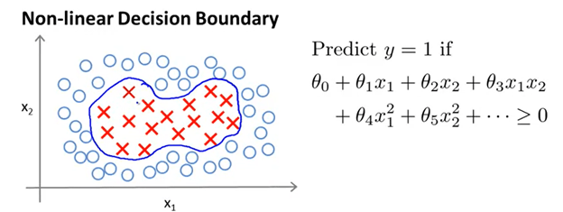
Again, we are really branching off past articles, so if you have not read up on logistic regression and the past SVM article, please do so! For this next lesson we are going to look at the possibility of including replacing the complex polynomial features in a cost function for the SVM. For example, in the figure below a non-linear decision boundary is created by utilizing x1^2 and x2^2. As you can tell, this instance is taken from linear regression with polynomial features. The hypothesis would be 1 if the equation is greater than or equal to 0. Otherwise, the hypothesis would be 0.
However, instead of saying x1, x2, x1^2, x2^2, it is possible to improve accuracy by replacing all the x’s with just f1, f2, f3, f4 etc. And the f1, f2, and f3 will be computed by finding the proximity of a given x to landmarks l1, l2, l3, etc. This is a bit hard to understand, so let us break this down with an example.

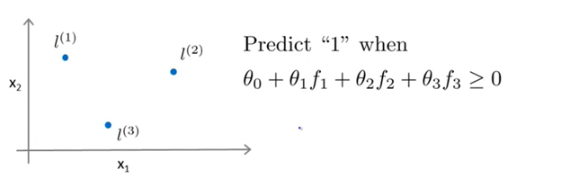
Here we randomly declared three landmarks in space and now instead of having complex polynomial features such as x1^2 * theta, we simply do f2*theta. In this specific case the formula we are using to calculate how close a x is to a specific landmark is called a Gaussian Kernel. It essentially takes the Euclidian distance from a point to a landmark and squares that. There is a regularization parameter which we will talk about later. If x is close to the landmark l1, then the Euclidean distance decreases and the inside term of the exp decreases. Because the Gaussian Kernel is indeed an exp (so essentially e raised to the power of something), when the inside term tends to 0, the function f1 becomes 1 and is maximized. Hence, when x is far away from a landmark, the inside term will tend to infinity and f2 will become 0.
Now observe the figure below
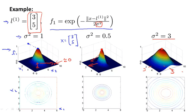
Here, the example declares one landmark that is at [3,5]. As you can see f1 is close to 1 if the x is close to [3,5], but one can change how “generous” f1 is. If the sigma is very small, then the algorithm will only spike to one if very specific x1 and x2 are reached. On the other hand, if the sigma is large, then the algorithm will be forgiving to those points which are not that close to [3,5].
The question still remains on how to accurately choose landmarks, which is something we will delve into next article. However, before we go over that, let me just conclude with an example.
Above, let us say theta0 is -0.5, theta1 is 1, theta2 is 1, and theta3 is 0 after gradient descent. There are still a bunch of questions that must arise such as how does the algorithm learn? How are the landmarks chosen? And yes, these answers will be answered in due time, but it is important to understand what this function is doing. So by theta3 being 0, the f3 feature does not matter. And only points near l1 and l2 will predict 1. Hence, the decision boundary created will be something similar to what follows:
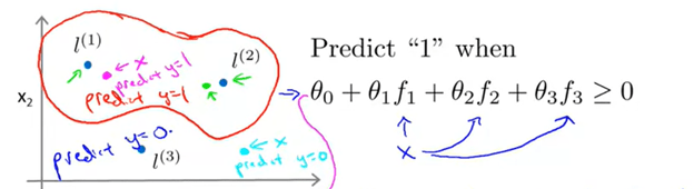
And now how fat or thin this decision boundary can be is decided by the sigma as explained in a couple paragraphs before. This is a little complex as it involves a deep understanding of both linear and logistic regression. If you keep reading, though, I will try my best to help you understand why SVMs are so powerful!
