Now that we learned about logistic regression, let us talk about support vector machines, also known as SVM’s. To gain more intuition behind the SVM, we are going to go back to our understanding of logistic regression. If you have not read those sets of articles, please do otherwise you will get lost.
Here is the formula for logistic regression again:
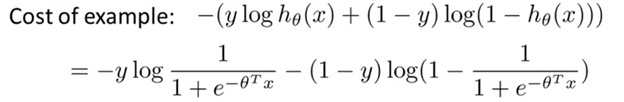
Remember that log(hypothesis) spikes up in cost when the hypothesis tends to 0, but the cost is 0 when the hypothesis is 1 because log(1) = 0. This is helpful if we are looking for the cost of an example where 1 is the desired value as the cost would increase at 0 but decrease at 1 (the same can be derived for log(1-h(x)).
If we were looking at a specific x and y example where the output we wanted is 1, our cost function graph would like this:
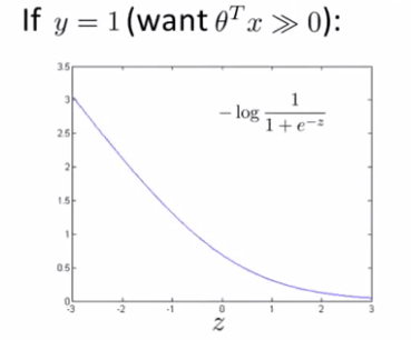
Where z is theta-transpose * x. In this case, we would want z to be extremely large, but now instead of having this curved line, we are going to make two straight lines so our cost function respect to z looks like:

By making these cost functions two straight lines, there will be a computationally easier classification task for the SVM (More on the advantages vs disadvantages will be discussed later). So now, using cost1 and cost0, our new cost formula becomes:

But for the SVM the notation calls a constant C = 1/lambda and the constant + regularization feature will look something like:

The output of the SVM differs from logistic regression as it makes a prediction of y = 1 or y = 0, there is no “probability”. If theta-transpose * x >= 0, once parameters theta have been learned, the SVM will output one. Otherwise it will output 0. Now let us move on to the individual hypothesis or cost1 cost0 functions in the equation.

In this example the left graph represents if y=1, we want z (theta-transpose * x) to be >= 1. The contrary is shown on the right we wants z to be <= -1. It is important to not that it is not just >= or <= 0, the SVM wants even more than that.
Now before we move on let us talk more about how this C affects the learning model. If we have a big C then the term on the equation needs to be as close to 0 as possible to offset the value of C, hence the model is more likely to overfit. However, if C is small (smaller than the regularization ½ * summation of thetatj^2) then there isn’t a big need to make the equation be very small and the model will not change that much with outliers (maybe even underfitting if C is too small).
Lets look back at what the SVM is offering to see why people use it. The best way to fully conceptualize the advantage is through a graph:

To separate the two sets of points above, decision boundaries like the green and orange lines may be made to achieve a perfect accuracy on the training data. However, it is evident that there is a cleaner solution if the slope of the line is less steep such as:

Here the black decision boundary is much more representative of the dataset and the distance between the boundary and the training examples is called the margin. Hence, sometimes the SVM is called the Large Margin Classifier. We will go into the mathematical intuition in further articles so sit tight!
(Sorry for the big break in between posting, will try and be more regular now)
