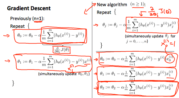
(Refer to Figure 1 first) Not a lot has changed from the last time we talked about gradient descent (please look at that article before reading on). It is hard to explain how the summation and 1/m comes into play, but when you take the partial derivative with respect to the variable that you are changing to the cost function you get the formula in the top right. This formula holds true for all cases even the base case because we set x0 to be 1 in all training examples because there is always a theta which does not have a x (for example y = thetax + theta). We say x0 is 1 because when we do theta transposed * elements of x the first element in the product matrix will be x0theta0 which is simplified to theta0.
To make gradient descent more efficient, it is ideal to have input values that have very similar values. For example instead of 1000, 2000, and 3000 as data points, having 1, 2, 3 would make it easier for gradient descent to take steps on. Ideally, -1< x(i) < 1 (the most common range of values in machine learning). Two ways to help with making the data manageable are mean normalization and feature scaling. Mean normalization is dividing each of the values by the mean, and the latter is dividing each value by the range. To combine both these strategies the formula below is adopted:
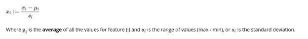
So if there are houses with a range of 200 dollars to 2200 dollars, a mean value of 1000, and a standard deviation of 2000 dollars, each value will be x-1000/2000. A house costing 1800 dollars will now be 0.4, and a house costing 600 dollars will be –0.2.

To stop gradient descent something called an automatic convergence test can be used. A “E” value (epsilon) can be determined that says if J(theta) decreases by less than this much, the performance gain is negligible and the algorithm should stop trying. In the Figure 3 epsilon can be 10^-3.

However, if the algorithm starts behaving weirdly and as the number of iterations goes up J(theta) does not go down, a couple problems could be apparent with your weights or biases. However, the main fix to this problem is to just make the learning rate small enough so the algorithm takes smaller incremented steps. As you can see on the right graph of Figure-4, comparing J(theta) and theta, there are two examples present: one with a bunch of small arrows and one with a few long arrows spanning the length of the parabola. The small arrows represent what happens if learning rate is decreased the algorithm will take much smaller steps. But if you look at the other example the learning rate is too much, and it overshoots the minimum by a great value. The slope at this new predicted point will be greater than what it was before so it increases theta by an even greater amount leading the algorithm to over shoot the minimum even more. This new very high theta has a steep slope, so it overshoots the minimum by even more by decreasing a great amount. This cycle keeps on going causing the j(theta) vs iterations curve to follow a e^x graph.
