Continuing from the last article to narrow down the theta1 and theta 0 we use a learning technique called gradient descent. So we have our cost function J(theta, theta1) and we want the result of the function to be the smallest possible. What gradient descent does is that it randomly starts with a theta and theta1, and it keeps changing the two variables until J(theta, theta1) reaches a minimum. If we go back to our 3-d graph we can get a better feel of what this algorithm is really doing (Example 1). First, the two random variables output a value on the top of a slope. The next step in this algorithm is to look all around the point and see which direction to go down. It goes down a certain amount (the specific length will be explained later), and repeats until it gets to a minimum.
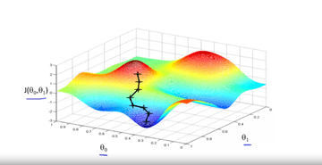
A problem you might notice with gradient descent is that if the algorithm randomly initialized on the other red hump, it would reach another minimum. However, most of the functions demonstrate a graph very similar to a bell shaped curve so there is a clear singular minimum. Now that we have a conceptual understanding let us talk about the math.

This function is basically saying that for each variable, simultaneously update the variables and plug it back into the formula. The alpha represents the learning rate of the algorithm. If the rate is very large then it takes big steps (leading the algorithm to overshoot the right value), or if the rate is very small then it takes very small steps (leading a large run time of the algorithm). The partial derivative is basically just the slope/rate of change of the curve. This is used because if the slope is positive then the equation become thetaj = thetaj – alpha * slope; hence, we would be decreasing the value. In the same vein, if our slope is negative, then we would increase the value of theta1 to get the slope as close as possible to 0. Our goal is to make derivative as small as possible, because when the derivative of a point is very small, that means that the point is a minimum on the graph J(theta) proving that the cost drops to a minimum at this point.
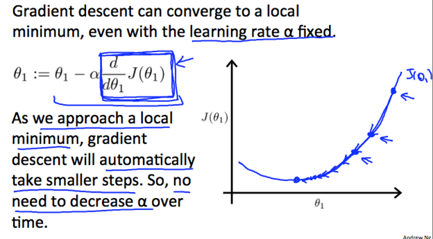
A great feature of gradient descent, is that even with a fixed learning rate (the constant alpha) the slope’s absolute value naturally decreases. What this means is that as the point gets closer and closer to the minimum the size of the step it will take will decrease to be more precise.
Now lets simplify the partial derivative of the cost function; the math is a little too advanced to detail but if you are looking for a derivation there is one below:
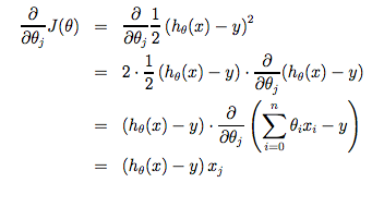
So now that we have the simplified version of the cost function we can plug that in, removing the partial derivative from our equation. The new equation for gradient descent becomes:

That is basically a good summary of gradient descent in a nutshell, it is a quite hard concept to grasp and hopefully as you keep on reading these articles the idea behind gradient descent makes sense. There are various types of gradient descent, but because all data is used in the tweaking of the theta this is called batch gradient descent.
